Limits and Continuity#
Limits of Sequences#
Understanding limits is absolutley crucial to understanding calculus, as they are the foundation of the entire subject. Let’s start by looking at the limits of sequences.
Def. A sequence of real numbers is a function \(x: \mathbb{N} \to \mathbb{R}\). The notation \(x_n\) is used to mean \(x(n)\), and a sequence is denoted \((x_n)_{n\in \mathbb{N}}\). A sequence \((x_n)_{n\in \mathbb{N}}\) is bounded if there is some \(M \geq 0 \) such that \(|x_n| \leq M \) for all \(n\in \mathbb{N}\). Otherwise \((x_n)_{n\in \mathbb{N}}\) is unbounded.
Let’s consider the sequence \(\left(\frac{1}{n}\right)_{n\in \mathbb{N}}\). This is the sequence \(1,1/2,/1/3,1/4...\) This sequence is bounded by \(1\). If we plot this sequence, we can see that it has interesting behavior:
import numpy as np
import matplotlib.pyplot as plt
N = np.arange(1,50,1)
plt.figure(figsize=(9,5))
plt.scatter(N,1/N);plt.title(r"$\left(\frac{1}{n}\right)_{n\in \mathbb{N}}$",fontsize = 20);plt.show()
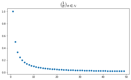
The values of this sequence seem to “approach” or get closer to \(0\) as \(n\) increases. Intuitivley, we can think that as \(n\) becomes large \(\frac{1}{n}\) becomes small since you are dividing by a bigger number. Note, however that no matter how big \(n\) gets, the value of the sequence will always be greater than zero, even though in some sense the sequence is “going to zero.”
To make this observation more precise, we introduce limits. In this case, we would write:
Limits capture the value sequences get arbitrarily close to as \(n\) becomes very large. It is worth noting here that not all sequences have limits, for example all unbounded sequences do not have limits.
This is very interesting but quite informal. What does “arbitrarily close” even mean? I’ll give the formal rigorous definition of limits of sequences next. You’ll probably never need to work with this definition directly as a physics major, but I do think it is extremely useful to know, as it gives a better way to think of limits.
Def. We say a sequence \((x_n)_{n\in \mathbb{N}}\) converges to \(x \in \mathbb{R}\) if for every \(\varepsilon > 0\) there exists \(N\in \mathbb{N}\) such that \(|x_n - x| < \varepsilon \) for all \(n\geq N\), and we write: \(\lim_{n\to\infty}x_n = x.\)
This is sayting that no matter how small of a value of \(\varepsilon\) you pick, you can always go out far enough in the sequence so that the value of the sequence is closer to its limit than whatever you chose \(\varepsilon\) to be.
But what about functions that have other imputs? These functions are more relevant to physics and we can extend our definition of limits to them.
Limits of other functions#
For functions \(f:S\to \mathbb{R}\), we can think of limits of the value of the function as x approaches some \(x \in S\) There are two ways that we can think of definining limits rigorously. The first is the formal \(\varepsilon\)-\(\delta\) definition which mimics the definition of convergence we’ve seen already. But in practice, that definition is not often used, so I’ll give the second version:
Theorem Let \(f:S\to \mathbb{R}\) be a function with \(S\subset \mathbb{R}\), and let \(x_0 \in S\), and let \(y_0\in \mathbb{R}\). Then \(\lim_{x\to x_0}f(x) = y_0\) if and only if for every sequence \((x_n)_{n\in\mathbb{N}} \subset S \setminus \{x_0\}\) converging to \(x_0\) one has that \((f(x_n))_{n\in\mathbb{N}}\) convergest to \(y_0\).
This essentially is saying that if you use a convergent sequence that converges to \(x_0\) as an imput for a function, the corresponding output sequence converges to the limit of the function.
Trick for finding limits of rational functions#
Let’s say you want to find the limit of the funciton \(f(x) = \frac{1 - 3x^2 + 3x^3}{x^3 -4x^2 -4}\) as \(x\to \infty\). Graphing the function, we can see that the limit should end up being \(3\):
x = np.arange(-3,40,0.1)
plt.figure(figsize=(9,5))
plt.plot(x,(1-3*x**2 + 3*x**3)/(x**3 - 4*x**2 + 4), label = r"$f(x) = \frac{1 - 3x^2 + 3x^3}{x^3 -4x^2 -4}$")
plt.plot(x,3*np.ones(len(x)), label = "g(x) = 3");plt.ylim(-10,10);plt.xlim(-2,x.max());plt.legend(fontsize = 15);plt.show()
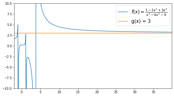
To be able to figure this out without graphing the function, there is a handy trick. Multiplying the denominator and numerator by \(\frac{1}{x^3}\) gives:
As x becomes large, all of the terms with powers of x in their denominators will go to zero, leaving behind \(\frac{3}{1} = 3\).
As you encounter various functions, you’ll learn their limiting behaviors. Exponentials come to mind as the other most important kind of function to understand the limits of. For example \(e^{-x}\) goes to \(0\) as \(x\to \infty\), and \(e^{1/x}\) goes to \(1\) in the same limit.
Continuity#
Most of the functions of interest in physics are continuous, or are at least mostly continuous. Intuitively, a function being continuous means that you can draw it without picking up your writing utensil.
Lets consider the function \(f(x) = \frac{1}{x}\) that is defined on \(\mathbb{R}\setminus \{0\}\). This function looks like this:
x1 = np.arange(-8,-0.01,0.05);x2 = np.arange(0.01,8,0.05)
plt.figure(figsize=(9,5))
plt.plot(x1,1/x1, c = 'b');plt.plot(x2,1/x2, c = 'b')
plt.title(r"$\frac{1}{x}$",fontsize = 20);plt.ylim(-10,10);plt.show()
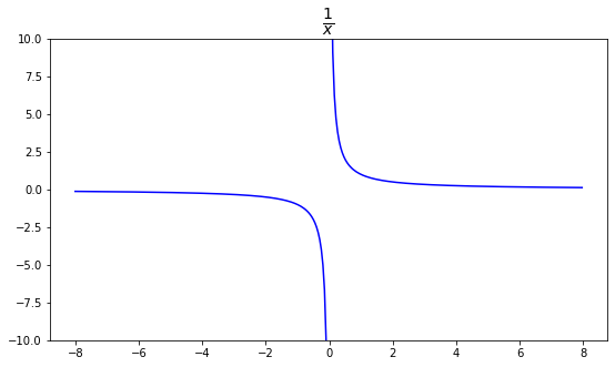
We can see that this function is continuous except at 0, where it isn’t even defined.
We are still lacking a solid definition of continuity. There is again a \(\varepsilon\) \(\delta\) formulation of this definition, but I’ll just give a more practical practical definition:
Def. Let \(f: S\to \mathbb{R}\) with \(S\subset\mathbb{R}\) and let \(x_0\in S\). \(f\) is continuous at \(x_0\) if and only if:
This is saying that if the limit of the function and its actual value at a point are the same, then the function is continuous at that point.